22.1 Sampling distribution: One mean with population standard deviation known

In this chapter, we study the situation where a population mean \(\mu\) (the parameter) is estimated by a sample mean \(\bar{x}\) (the statistic).

Of course, every sample is likely to be different, and is likely to produce a different sample mean \(\bar{x}\). That is, the value of the sample mean will vary from sample to sample and exhibit sampling variation (which can be quantified using the standard error).

Consider rolling dice again. Suppose a die is rolled \(n=25\) times, and the mean of the 25 numbers that are rolled is recorded. What will be the sample mean of the numbers in the 25 rolls?

The sample mean will vary from sample to sample, (sampling variation). Since every face of the die is equally likely to appear on any one roll, the population mean of all possible rolls is \(\mu=3.5\) (in the middle of the numbers on the faces of the die, which is also the median).

An example of the mean after repeatedly rolling a die 25 times is shown in the animation below for 10 sets of 25 rolls. The mean of the 25 rolls clearly varies. In the simulation, the sample mean of 25 rolls was as low as 3.08 and as high as 3.76.

The mean for any single sample of \(n=25\) rolls will sometimes be higher than \(\mu=3.5\), and sometimes lower than \(\mu=3.5\), but most of the time the mean should be close to 3.5.

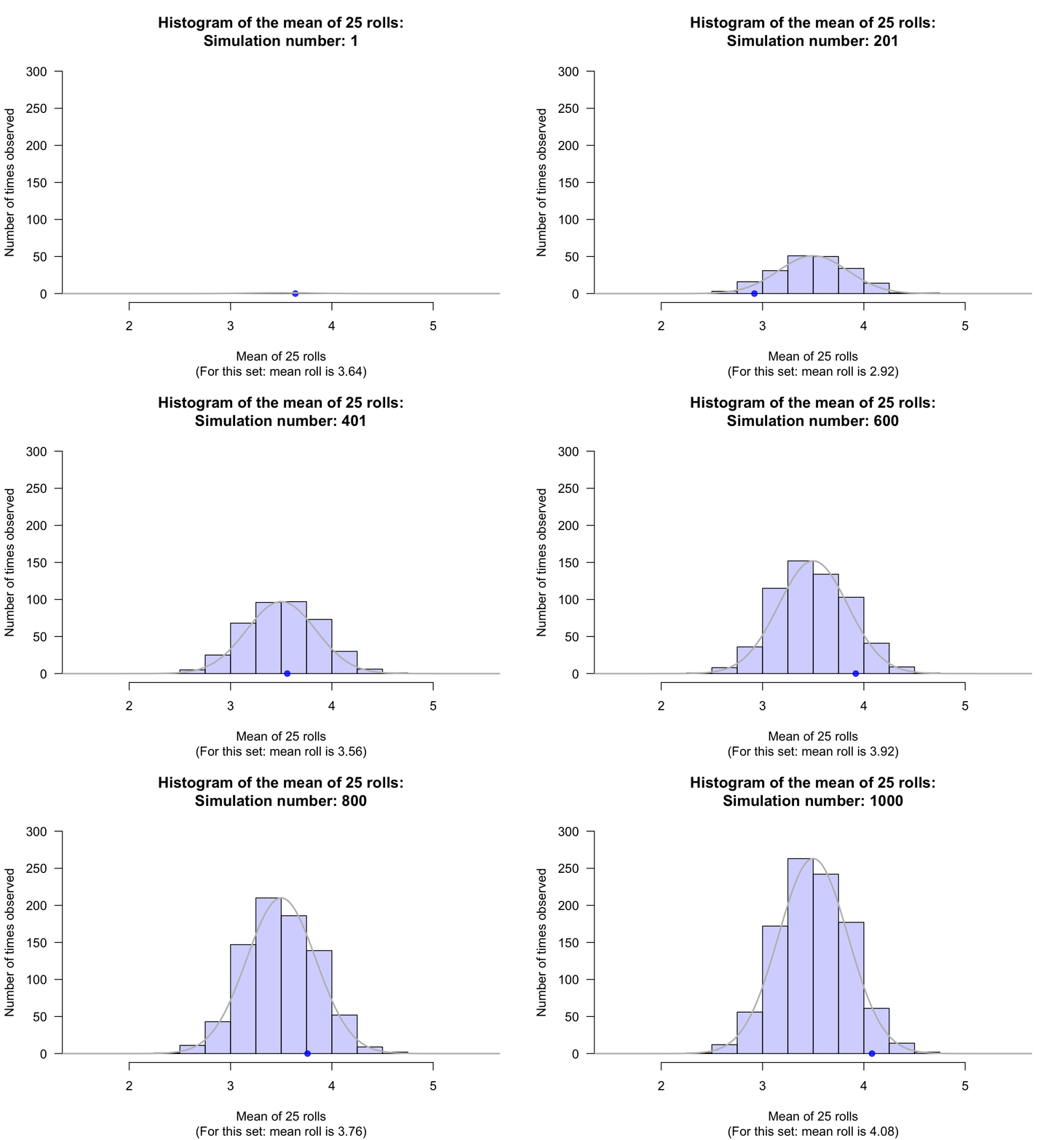
If many people made a set of 25 rolls, and computed the mean for their set, every person would have a sample mean for their set of 25 rolls, and we could produce a histogram of all these sample means; see the animation below.

From the animation above, the sample means appear to vary with an approximate normal distribution (as we saw with the sample proportions). This normal distribution is centred around the population mean \(\mu\). The standard deviation of the normal distribution is the standard error of the sample mean \(\bar{x}\), written as \(\text{s.e.}(\bar{x})\).

When the population standard deviation \(\sigma\) is known, then

\[ \text{s.e.}(\bar{x}) = \frac{\sigma}{\sqrt{n}}. \] So the possible values of the sample means have a sampling distribution described by:

• an approximate normal distribution,
• with mean \(\mu\), and
• a standard deviation, called the standard error, of \(\text{s.e.}(\bar{x}) = \sigma/\sqrt{n}\).

Usually the population mean and the population standard deviation are unknown. Nonetheless, because the sampling distribution has an approximate normal distribution, the 68–95–99.7 rule can be applied: approximately 95% of the sample means are expected to be within two standard errors of \(\mu\).