35.2 Linear equations: A review

An example of a regression equation is

$\hat{y} = - 4 + 2 x .$ Here, $x$ refers to the explanatory variable, $y$ refers to the observed response variable, and $\hat{y}$ refers to the predicted values of the response variable.

In general, the equation of a straight line is written as

$\hat{y} = b_{0} + b_{1} x$ where $b_{0}$ and $b_{1}$ are just numbers. Again, $\hat{y}$ refers to the predicted (not observed) values of $y$ .

\hat{y}

is pronounced as ‘why hat’; the ‘caret’ above the

y

is called a ‘hat,’ and designates a predicted value (of

y

Example 35.1 (Regression equations) In the regression equation

\hat{y} = 15 - 102 x

, we have

b_{0} = 15

and

b_{1} = - 102

Think 35.1 (Regression coefficients) Consider the regression equation

\hat{y} = 0.0047 x + 2.1

. What are the values of

b_{0}

and

b_{1}

? (Look carefully!)

In this case,

b_{0} = 2.1

and

b_{1} = - 0.0047

. Remember that

b_{1}

is the number multiplied by the

x

, and that

b_{0}

is the number by itself. Some software and some journal papers write regression equations with the value of

b_{0}

first, and some with the value of

b_{1}

first. It’s not the order that’s important.

The numbers $b_{0}$ and $b_{1}$ are called regression coefficients, where

$b_{0}$ is a number called the intercept. It is the predicted value of $y$ when $x = 0$ .
$b_{1}$ is a number called the slope. It is, on average, how much the value of $y$ changes when the value of $x$ increases by 1.

We will use software to find the values of $b_{0}$ and $b_{1}$ . However, we can roughly guess the values of the intercept by first drawing what looks like a sensible straight line through the data, and determining what that line predicts for the value of $y$ when $x = 0$ .

A rough guess of the slope can be made using the formula

$slope = \frac{Change in y}{Corresponding change in x} = \frac{rise}{run} .$ That is, a guess of the slope is the change in the value of $y$ (the ‘rise’) divided by the corresponding change in the value of $x$ (the ‘run’).

To demonstrate, consider the scatterplot in Fig. 35.1. I have drawn a sensible line on the graph to capture the relationship (your line may look a bit different). When $x = 0$ , the regression line predicts the value of $y$ is about to be 2, so $b_{0}$ is approximately 2.

To guess the slope, use the ‘rise over run’ idea. The animation below may help explain the rise-over-run idea. When the value of $x$ increases from 1 to 5 (a change of $5 - 1 = 4$ ), the corresponding values of $y$ change from 5 to 17 (a change of $17 - 5 = 12$ ). Then, use the formula:

$\begin{aligned} \frac{rise}{run} & = \frac{17 - 5}{5 - 1} \\ = \frac{12}{4} = 3. \end{aligned}$ The value of $b_{1}$ is about $3$ . The regression line is approximately $\hat{y} = 2 + (3 \times x)$ , usually written as

$\hat{y} = 2 + 3 x .$

The intercept has the same measurement units as the response variable. For example, with the red-deer data the intercept is measured in ‘grams,’ the measurement units of the molar weight.

The measurement unit for the slope is the ‘measurement units of the response variable,’ per ‘measurement units of the explanatory variable.’ For example, with the red-deer data the slope has the units of ‘grams per year.’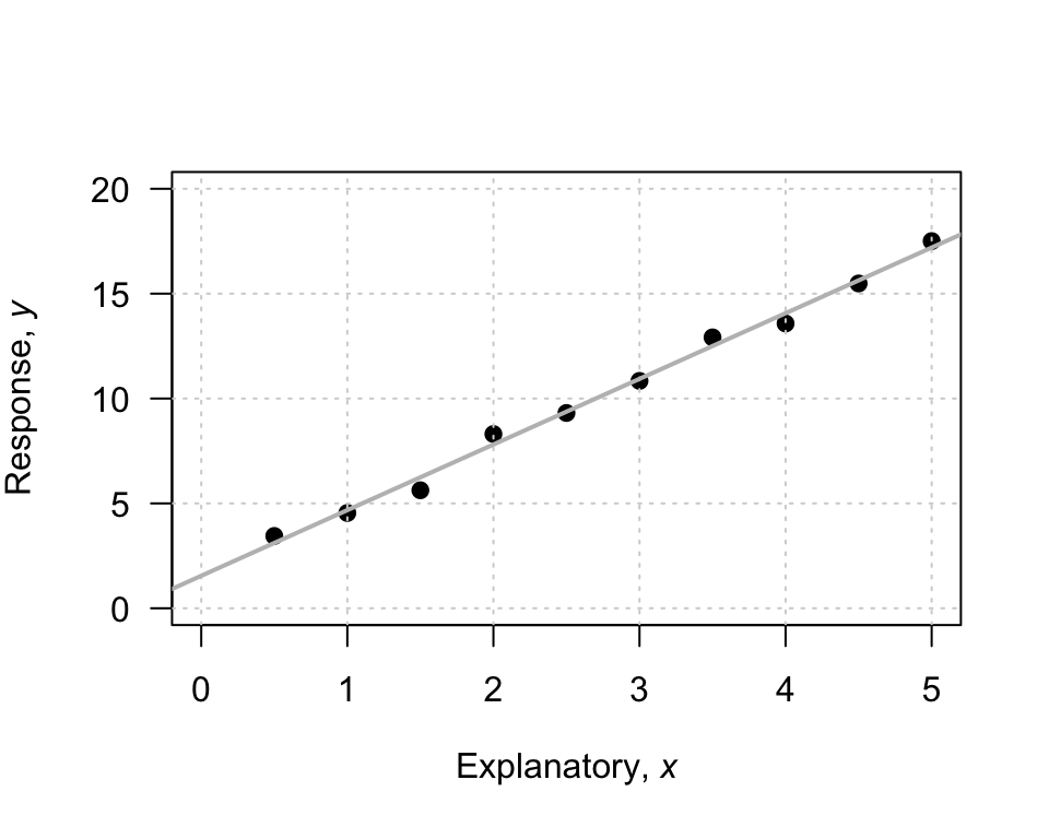

FIGURE 35.1: An example scatterplot

Example 35.2 (Estimating regression parameters) A study (Dunn and Smyth 2018) examined the number of cyclones $y$ in the Australian region each year from 1969 to 2005, and the relationship with a climatological index called the Ocean Nino Index (ONI, $x$ ); see (Fig. 35.2),

When the value of $x$ is zero, the predicted value of $y$ is about 12; $b_{0}$ is about 12. (You may get something slightly different.) Notice that the intercept is the predicted value of $y$ when $x = 0$ , which is not at the left of the graph.

To guess the value of $b_{1}$ , use the ‘rise over run’ idea. When $x$ is about $- 2$ , the predicted value of $y$ is about 17. When $x$ is about $2$ , the predicted value of $y$ is about 8. So when the value of $x$ changes by $2 - (- 2) = 4$ , the value of $y$ changes by $8 - 17 = - 9$ (a decrease of about 9). Hence, the value of $b_{1}$ is approximately $- 9 / 4 = - 2.25$ . (You may get something slightly different.) Notice that the relationship has a negative direction, so the slope must be negative.

Using these guesses of $b_{0} = 12$ and $b_{1} = - 2.25$ , the regression line is approximately $\hat{y} = 12 - 2.25 x .$

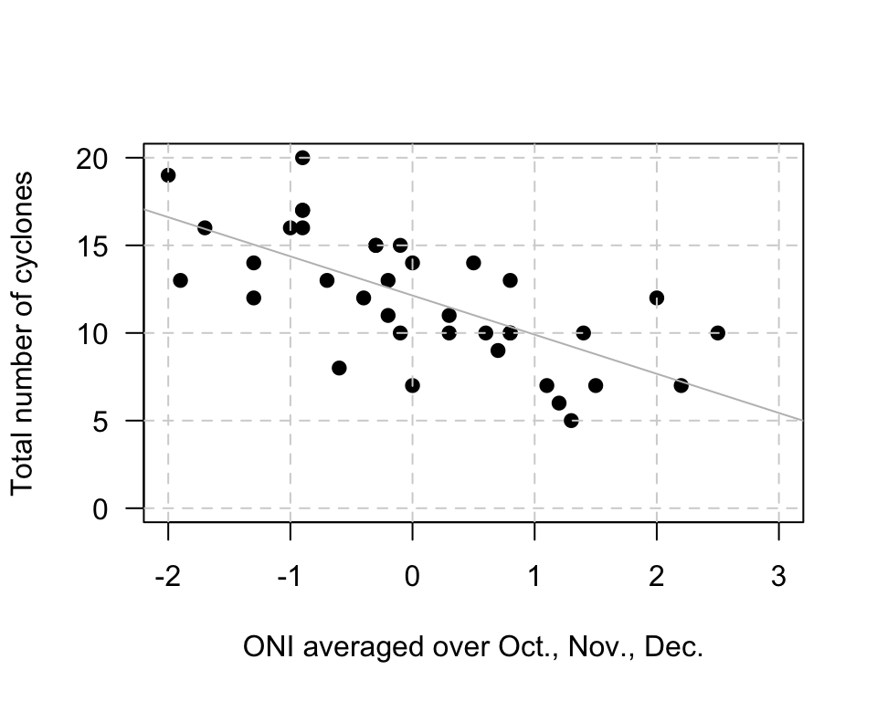
FIGURE 35.2: The number of cyclones in the Australian region each year from 1969 to 2005, and the ONI for October, November, December

In this section, we have seen how to understand a linear regression equation, and how an equation can be used to describe a fitted line. The above method gives a very crude guess of the values of the intercept $b_{0}$ and the slope $b_{1}$ . In practice, many reasonable lines could be drawn through a scatterplot of data. However, one of those lines is the ‘best fitting line’ in some sense¹⁸. Software calculates this ‘line of best fit’ for us.

For those who want to know: The ‘line of best fit’ is the line such that the sum of the squared vertical distances between the observations and the line is as small as possible.↩︎