18.2 Sample proportions have a distribution

As with any sample statistic, sample proportions vary from sample to sample (Sect. 15.4); that is, sampling variation exists, so the sample proportions have a sampling distribution.

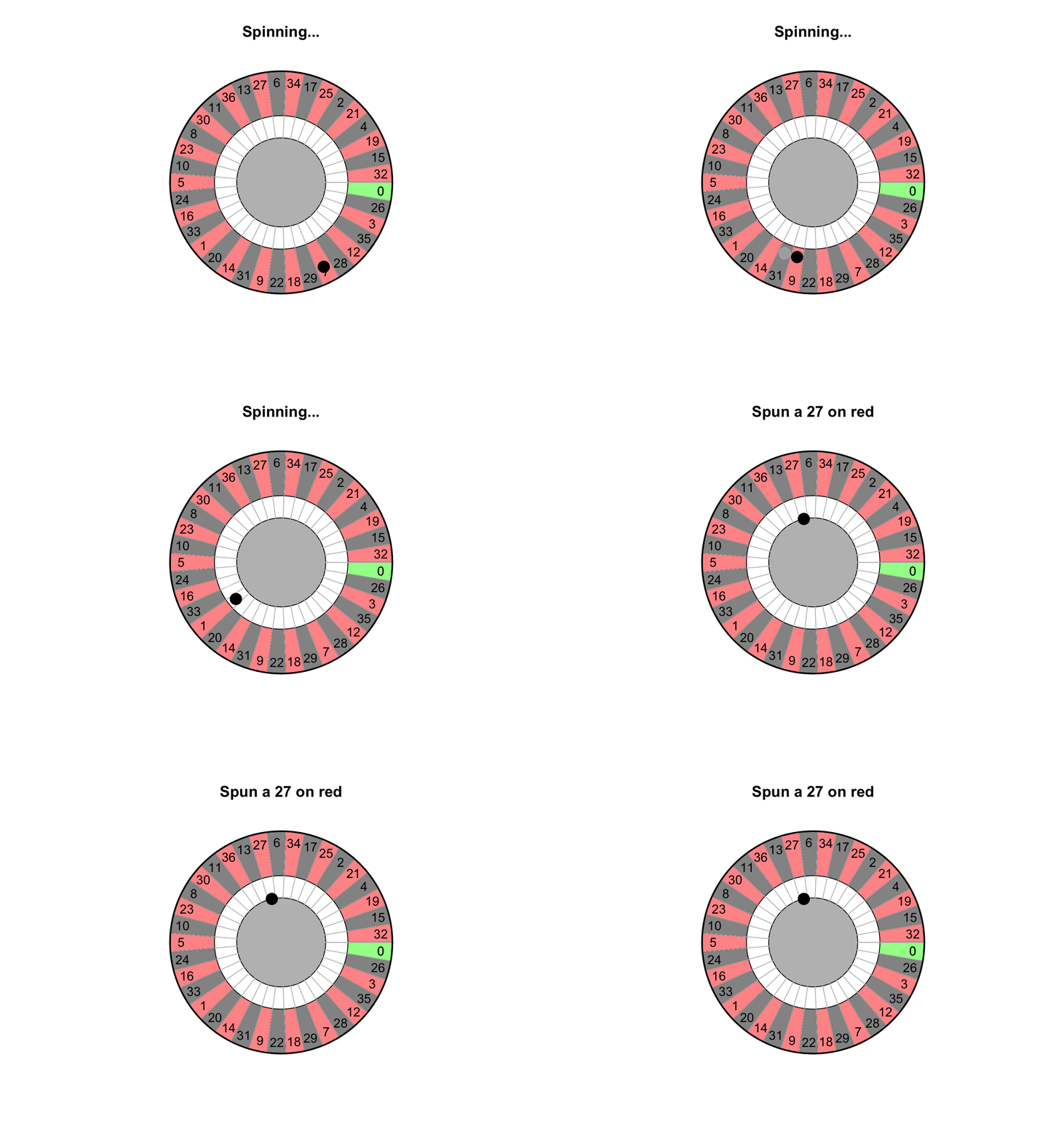
Consider a European roulette wheel shown below in the animation: a ball is spun and can land on any number on the wheel from 0 to 36 (inclusive).

Using the classical approach to probability, the probability of the ball landing on an odd number (an ‘odd-spin’) is \(p = 18/37 = 0.486\). However, if the wheel is spun (say) 15 times, the sample proportion of odd-spins \(\hat{p}\) can vary. Of course, the sample proportion \(\hat{p}\) of odd-spins can vary after spinning the wheel 30, 50 or 100 times also. How does it vary from spin to spin?

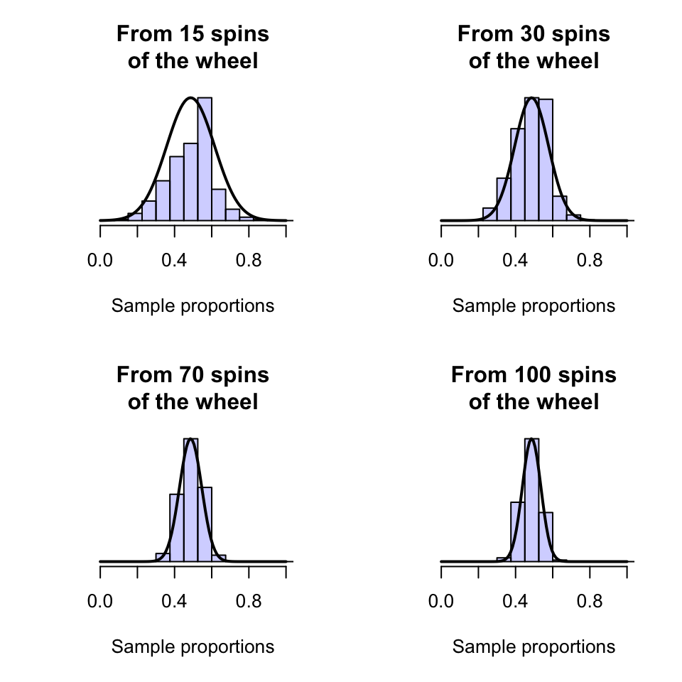
Computer simulation can be used to demonstrate what happens if the wheel was spun \(n=15\) times, over and over and over again, and the proportion of odd-spins was recorded for each repetition. Clearly, the proportion of odd spins \(\hat{p}\) can vary from sample to sample (sampling variation) for \(n=15\) spins, as shown by the histogram (Fig. 18.1, top left panel).

If the wheel was spun (say) \(n=40\) times, something similar occurs (Fig. 18.1, top right panel): the values of \(\hat{p}\) vary from sample to sample.

The same process can be repeated for (say) \(n=70\) and \(n=100\) spins (Fig. 18.1, bottom panels). Notice that as the sample size \(n\) gets larger, the distribution of the values of \(\hat{p}\) look more like an approximate normal distribution, and the variation gets smaller.

FIGURE 18.1: Sampling distributions for the proportion of roulette wheel spins that show an odd number

The values of the sample proportion vary from sample to sample. The distribution of the possible values of the sample statistic (in this case the sample proportion) from sample to sample is called a sampling distribution.

Under certain conditions, the sampling distribution of a sample proportion is described by an approximate a normal distribution. In general, the approximation gets better as the sample size gets larger.