15.4 Making decisions in research
Let’s think about each step in the decision-making process (Fig. 15.1) individually.
15.4.1 Assumption about the population parameter
![]()
Usually a reasonable assumption can be made about the population parameter. For example:
We might assume that no difference exists between the parameter for two groups in the population, since we don’t have any evidence yet to say there is a difference.
For example, we might assume that the mean HDL cholesterol (or the odds of a diabetes diagnosis) is the same for current smokers and non-smokers in the population, for the NHANES data. If we already knew there was a difference, why would we be performing a study to see if there is a difference?We might be interested in testing a claim, or evaluating a benchmark, about a population parameter, to determine if the evidence supports this claim or benchmark,
These assumptions about the population parameter are called null hypotheses.

Example 15.2 (Assumptions about the population) Most dental associations, such as the American Dental Association and the Australian Dental Association, recommend brushing teeth for two minutes. One study (I. D. M. Macgregor and Rugg-Gunn 1979) recorded the tooth-brushing time for 85 uninstructed schoolchildren (11 to 13 years old) from England.
We could assume the population mean tooth-brushing time in the population (‘school children (11 to 13 years old) from England’) is two minutes, as recommended. After all, we don’t have evidence to suggest any other value for the mean. A sample can then be obtained to determine if the sample mean is consistent with, or contradicts, this assumption.15.4.2 Expectations of sample statistics
![]()
Having made an assumption about the population parameter, the second step is to determine what values to expect from the sample statistic, based on this assumption.
Since every sample is likely to be different (‘sampling variation’, the value of the sample statistic depends on which of the possibe samples we end up with: the sample statistic is likely to be different for every sample.
Think about the cards in Sect. 15.2. Assuming a fair pack, then half the cards are red in the population (the pack of cards), so the population proportion is assumed to be \(p=0.5\).
In a sample of 15 cards, what values could be reasonably expected for the sample proportion \(\hat{p}\) of red cards (the statistic)? If samples of size 15 were repeatedly taken, the sample proportion of red cards would vary from hand to hand, of course.
How much would \(\hat{p}\) vary from sample to sample? Perhaps 15 red cards out of 15 cards happens reasonably frequently. Or perhaps it doesn’t. How could we find out? We could:
- Use mathematical theory to determine how likely it is that we would get 15 red cards out of 15 cards.
- We could repeatedly shuffle a pack of cards, and repeatedly deal 15 cards many hundreds or thousands of times, then compute how often we get 15 red cards of out 15 cards.
- More reasonably, we could simulate (using a computer) dealing 15 cards many hundreds or thousands of times, and count how often we get 15 red cards of out 15 cards.
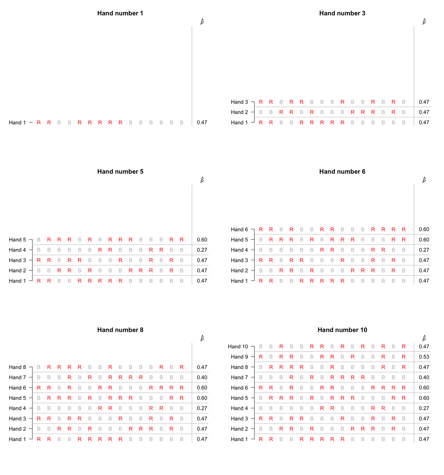
The third option is the most practical… To begin, suppose we simulated only ten hands of 15 cards each; the animation below shows the sample proportion of red cards from ten repetitions. Not one of those ten hands produced 15 red cards in 15 cards.

Suppose we repeated this for hundreds of hands of 15 cards, and for each hand we recorded the sample proportion of cards that were red. The proportion of red cards would vary from sample to sample (‘sampling variation’), and we could record the proportion of red cards from each of those hundreds of hands.
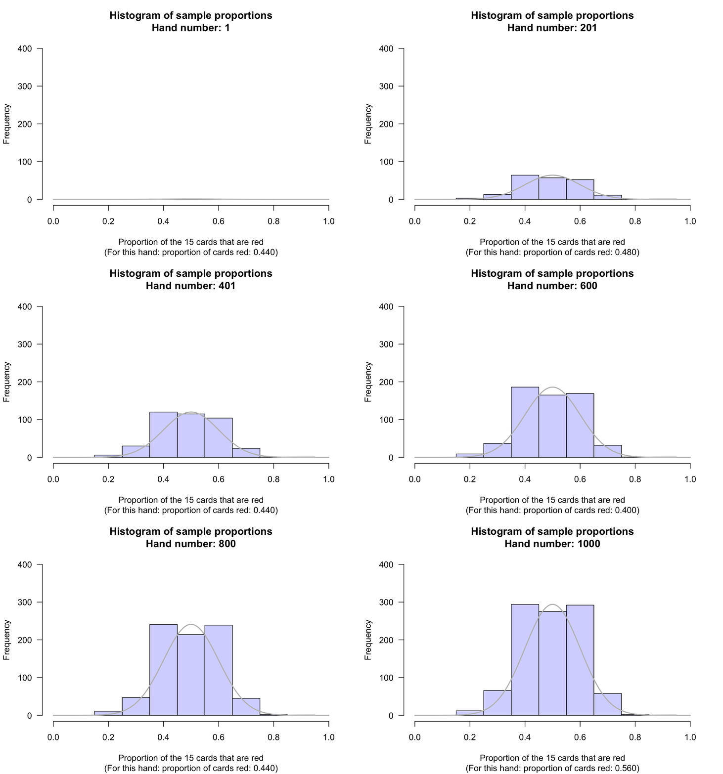
For these hundreds of sample proportions, we could draw a histogram; for example, the animation below shows a histogram of the sample proportions from 1000 repetitions of a hand of 15 cards.
This histogram shows how we might expect the sample proportions \(\hat{p}\) to vary from sample to sample, when the population proportion of red cards is \(p=0.5\).
We can see that observing 15 red cards out of 15 cards is quite rare: it never happened once in the 1000 simulations.

15.4.3 Observations about our sample
![]()
From this histogram, based on a simulation of one thousand hands, we could conclude that we would almost never find 15 red cards in 15 cards… if the assumption of a fair pack was true. But we did find 15 red cards in 15 cards… so the assumption (‘a fair pack’) is probably wrong.
What if we had observed 4 red cards in a hand of 15 cards (a sample proportion of \(\hat{p} = 4/15 = 0.267\)), rather than 15 red cards out of 15? The conclusion is not quite so obvious then: these values of \(\hat{p}\) are uncommon, but they certainly do happen when \(p=0.5\). In these situations, a more sophisticated approach for making a decision is needed.
Special tools are needed to describe what to expect from the sample statistic after making assumptions about the population parameter. These special tools are discussed in the next chapter.

Example 15.3 (Sampling variation) Most dental associations, such as the American Dental Association and the Australian Dental Association, recommend brushing teeth for two minutes. One study (I. D. M. Macgregor and Rugg-Gunn 1979) recorded the tooth-brushing time for 85 uninstructed schoolchildren from England (11 to 13 years old).
The sample mean tooth-brushing time may or may not be two minutes. Of course, every possible sample of 85 children will include different children, and so produce a different sample mean \(\bar{x}\). Even if the population mean toothbrushing time really is two minutes (\(\mu=2\)), the sample mean probably won’t be exactly two minutes, because of sampling variation.
We could assume the population mean tooth-brushing time is two minutes (\(\mu=2\)). If this assumption is true, we then could describe what values of the sample statistic \(\bar{x}\) to expect. Then, after obtaining a sample and computing the sample mean, we could determine if the sample mean seems consistent with the assumption of two minutes, or whether it seems to contradict this assumption.